Accelerated Geometry Probability Probability Test Review Conditional Probability P(Physics English)

Probability of an effect occurring, given that some other event has already occurred

In probability theory, conditional probability is a measure of the probability of an event occurring, given that another event (by assumption, presumption, exclamation or evidence) has already occurred.^[1] This item method relies on upshot B occurring with some sort of relationship with another result A. In this event, the outcome B can be analyzed by a conditionally probability with respect to A. If the event of interest is A and the event B is known or assumed to have occurred, "the conditional probability of A given B", or "the probability of A nether the condition B", is usually written as P(A|B) ^[two] or occasionally P _B (A). This can also be understood every bit the fraction of probability B that intersects with A: ${\displaystyle P(A\mid B)={\frac {P(A\cap B)}{P(B)}}}$ .^[3]

For example, the probability that whatever given person has a cough on any given twenty-four hours may exist but 5%. Simply if we know or presume that the person is sick, then they are much more probable to be coughing. For instance, the conditional probability that someone unwell (sick) is coughing might be 75%, in which case we would have that P(Cough) = v% and P(Cough|Sick) = 75%. Although in that location is a human relationship between A and B in this example, such a relationship or dependence between A and B is non necessary, nor do they have to occur simultaneously.

P(A|B) may or may non be equal to P(A) (the unconditional probability of A). If P(A|B) = P(A), then events A and B are said to be independent: in such a example, knowledge about either event does not alter the likelihood of each other. P(A|B) (the provisional probability of A given B) typically differs from P(B|A). For example, if a person has dengue fever, the person might have a 90% chance of existence tested as positive for the illness. In this case, what is beingness measured is that if event B (having dengue) has occurred, the probability of A (tested as positive) given that B occurred is xc%, merely writing P(A|B) = 90%. Alternatively, if a person is tested as positive for dengue fever, they may have simply a xv% adventure of actually having this rare disease due to high false positive rates. In this case, the probability of the outcome B (having dengue) given that the upshot A (testing positive) has occurred is 15% or P(B|A) = 15%. It should exist apparent now that falsely equating the two probabilities can lead to various errors of reasoning, which is normally seen through base of operations rate fallacies.

While conditional probabilities tin can provide extremely useful information, limited information is often supplied or at hand. Therefore, it tin can be useful to opposite or convert a condition probability using Bayes' theorem: ${\displaystyle P(A|B)={{P(B|A)*P(A)} \over {P(B)}}}$ .^[iv] Another option is to brandish conditional probabilities in provisional probability table to illuminate the human relationship betwixt events.

Definition [edit]

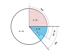
Illustration of conditional probabilities with an Euler diagram. The unconditional probability P(A) = 0.30 + 0.10 + 0.12 = 0.52. Still, the conditional probability P(A|B ₁) = ane, P(A|B _ii) = 0.12 ÷ (0.12 + 0.04) = 0.75, and P(A|B ₃) = 0.

On a tree diagram, branch probabilities are conditional on the event associated with the parent node. (Here, the overbars indicate that the event does not occur.)

Venn Pie Nautical chart describing provisional probabilities

Workout on an event [edit]

Kolmogorov definition [edit]

Given two events A and B from the sigma-field of a probability space, with the unconditional probability of B being greater than nada (i.due east., P(B) > 0), the conditional probability of A given B ( ${\displaystyle P(A\mid B)}$ ) is the probability of A occurring if B has or is assumed to take happened.^[5] A is assumed to a set of all possible outcomes of an experiment or random trial that has a restricted or reduced sample space. The conditional probability tin can exist constitute by the quotient of the probability of the articulation intersection of events A and B ( ${\displaystyle P(A\cap B)}$ ) -- the probability at which A and B occur together, although not necessarily occurring at the same time-- and the probability of B:^{[2] [6] [7]}

${\displaystyle P(A\mid B)={\frac {P(A\cap B)}{P(B)}}}$ .

For a sample space consisting of equal likelihood outcomes, the probability of the outcome A is understood as the fraction of the number of outcomes in A to the number of all outcomes in the sample infinite. Then, this equation is understood every bit the fraction of the set ${\displaystyle A\cap B}$ to the set B. Note that the above equation is a definition, non but a theoretical result. Nosotros denote the quantity ${\displaystyle {\frac {P(A\cap B)}{P(B)}}}$ as ${\displaystyle P(A\mid B)}$ and call it the "provisional probability of A given B."

As an axiom of probability [edit]

Some authors, such as de Finetti, adopt to introduce conditional probability equally an axiom of probability:

${\displaystyle P(A\cap B)=P(A\mid B)P(B)}$ .

This equation for a conditional probability, although mathematically equivalent, may be intuitively easier to sympathise. Information technology can be interpreted as "the probability of B occurring multiplied by the probability of A occurring, provided that B has occurred, is equal to the probability of the A and B occurrences together, although non necessarily occurring at the same time". Additionally, this may be preferred philosophically; under major probability interpretations, such equally the subjective theory, conditional probability is considered a primitive entity. Moreover, this "multiplication rule" can be practically useful in computing the probability of ${\displaystyle A\cap B}$ and introduces a symmetry with the summation axiom for mutually exclusive events:^[8]

${\displaystyle P(A\cup B)=P(A)+P(B)-P(A\cap B)}$

Thus the equations can be combined to find a new representation of the :

${\displaystyle P(A\cap B)=P(A)+P(B)-P(A\loving cup B)=P(A\mid B)P(B)}$

${\displaystyle P(A\cup B)={P(A)+P(B)-P(A\mid B){P(B)}}}$

As the probability of a provisional event [edit]

Provisional probability tin be divers as the probability of a conditional outcome ${\displaystyle A_{B}}$ . The Goodman–Nguyen–Van Fraassen conditional event can be defined as:

${\displaystyle A_{B}=\bigcup _{i\geq i}\left(\bigcap _{j<i}{\overline {B}}_{j},A_{i}B_{i}\right)}$ , where ${\displaystyle A_{i}}$ and ${\displaystyle B_{i}}$ stand for states or elements of A or B. ^[9]

It can be shown that

${\displaystyle P(A_{B})={\frac {P(A\cap B)}{P(B)}}}$

which meets the Kolmogorov definition of conditional probability.^[x]

Conditioning on an result of probability zero [edit]

If ${\displaystyle P(B)=0}$ , and then co-ordinate to the definition, ${\displaystyle P(A|B)}$ is undefined.

The instance of greatest interest is that of a random variable Y, conditioned on a continuous random variable X resulting in a particular outcome x. The event ${\displaystyle B=\{X=x\}}$ has probability zero and, as such, cannot exist conditioned on.

Instead of conditioning on Ten being exactly ten, we could condition on it existence closer than distance ${\displaystyle \epsilon }$ away from x. The event ${\displaystyle B=\{x-\epsilon <X<x+\epsilon \}}$ volition generally have nonzero probability and hence, can be conditioned on. We can and then have the limit

${\displaystyle \lim _{\epsilon \to 0}P(A\mid x-\epsilon <X<x+\epsilon ).}$

For instance, if two continuous random variables X and Y have a articulation density ${\displaystyle f_{X,Y}(x,y)}$ , then by L'Hôpital's rule and Leibniz integral rule, upon differentiation with respect to ${\displaystyle \epsilon }$ :

${\displaystyle {\begin{aligned}\lim _{\epsilon \to 0}P(Y\in U\mid x_{0}-\epsilon <X<x_{0}+\epsilon )&=\lim _{\epsilon \to 0}{\frac {\int _{x_{0}-\epsilon }^{x_{0}+\epsilon }\int _{U}f_{X,Y}(10,y)\mathrm {d} y\mathrm {d} x}{\int _{x_{0}-\epsilon }^{x_{0}+\epsilon }\int _{\mathbb {R} }f_{X,Y}(10,y)\mathrm {d} y\mathrm {d} x}}\\&={\frac {\int _{U}f_{10,Y}(x_{0},y)\mathrm {d} y}{\int _{\mathbb {R} }f_{Ten,Y}(x_{0},y)\mathrm {d} y}}.\terminate{aligned}}}$

The resulting limit is the conditional probability distribution of Y given X and exists when the denominator, the probability density ${\displaystyle f_{X}(x_{0})}$ , is strictly positive.

It is tempting to ascertain the undefined probability ${\displaystyle P(A|X=x)}$ using this limit, but this cannot be done in a consistent fashion. In item, it is possible to find random variables Ten and W and values ten, due west such that the events ${\displaystyle \{Ten=x\}}$ and ${\displaystyle \{W=westward\}}$ are identical but the resulting limits are non:^[11]

${\displaystyle \lim _{\epsilon \to 0}P(A\mid 10-\epsilon \leq Ten\leq x+\epsilon )\neq \lim _{\epsilon \to 0}P(A\mid w-\epsilon \leq W\leq w+\epsilon ).}$

The Borel–Kolmogorov paradox demonstrates this with a geometrical argument.

Workout on a discrete random variable [edit]

Allow X be a discrete random variable and its possible outcomes denoted 5. For instance, if 10 represents the value of a rolled die then V is the set ${\displaystyle \{1,two,3,iv,five,half-dozen\}}$ . Allow u.s.a. presume for the sake of presentation that Ten is a discrete random variable, so that each value in V has a nonzero probability.

For a value x in V and an event A, the conditional probability is given past ${\displaystyle P(A\mid X=x)}$ . Writing

${\displaystyle c(ten,A)=P(A\mid X=x)}$

for short, we run across that it is a function of two variables, 10 and A.

For a fixed A, we can form the random variable ${\displaystyle Y=c(X,A)}$ . It represents an consequence of ${\displaystyle P(A\mid X=x)}$ whenever a value x of Ten is observed.

The conditional probability of A given X tin can thus be treated as a random variable Y with outcomes in the interval ${\displaystyle [0,1]}$ . From the police of total probability, its expected value is equal to the unconditional probability of A.

Partial conditional probability [edit]

The partial conditional probability ${\displaystyle P(A\mid B_{i}\equiv b_{1},\ldots ,B_{1000}\equiv b_{thousand})}$ is about the probability of event ${\displaystyle A}$ given that each of the status events ${\displaystyle B_{i}}$ has occurred to a caste ${\displaystyle b_{i}}$ (degree of belief, caste of experience) that might be different from 100%. Frequentistically, fractional conditional probability makes sense, if the conditions are tested in experiment repetitions of advisable length ${\displaystyle n}$ .^[12] Such ${\displaystyle n}$ -bounded partial conditional probability tin can be divers as the conditionally expected boilerplate occurrence of outcome ${\displaystyle A}$ in testbeds of length ${\displaystyle n}$ that attach to all of the probability specifications ${\displaystyle B_{i}\equiv b_{i}}$ , i.e.:

${\displaystyle P^{n}(A\mid B_{one}\equiv b_{one},\ldots ,B_{m}\equiv b_{m})=\operatorname {E} ({\overline {A}}^{due north}\mid {\overline {B}}_{1}^{northward}=b_{1},\ldots ,{\overline {B}}_{m}^{n}=b_{thousand})}$ ^[12]

Based on that, partial conditional probability tin be defined as

${\displaystyle P(A\mid B_{1}\equiv b_{i},\ldots ,B_{m}\equiv b_{chiliad})=\lim _{due north\to \infty }P^{north}(A\mid B_{1}\equiv b_{1},\ldots ,B_{m}\equiv b_{g}),}$

where ${\displaystyle b_{i}northward\in \mathbb {North} }$ ^[12]

Jeffrey conditionalization^{[13] [fourteen]} is a special case of fractional provisional probability, in which the status events must class a partition:

${\displaystyle P(A\mid B_{i}\equiv b_{i},\ldots ,B_{yard}\equiv b_{m})=\sum _{i=ane}^{m}b_{i}P(A\mid B_{i})}$

Example [edit]

Suppose that somebody secretly rolls two fair 6-sided dice, and nosotros wish to compute the probability that the face-up value of the kickoff one is 2, given the information that their sum is no greater than 5.

• Let D ₁ be the value rolled on dice i.
• Let D ₂ be the value rolled on die 2.

Probability that D ₁ = 2

Table 1 shows the sample space of 36 combinations of rolled values of the two dice, each of which occurs with probability 1/36, with the numbers displayed in the red and dark gray cells being D ₁ + D ₂.

D ₁ = 2 in exactly half dozen of the 36 outcomes; thus P(D ₁ = ii) = 6⁄36  = 1⁄6 :

Table 1

+		Dtwo
		one	ii	3	4	5	half dozen
D 1	1	2	3	4	five	half dozen	7
	2	3	4	5	6	vii	8
	3	4	v	6	seven	8	9
	iv	5	6	7	8	9	10
	5	6	7	eight	9	10	11
	6	7	viii	9	10	11	12

Probability that D _ane +D ₂ ≤ v

Table 2 shows that D ₁ +D _two ≤ 5 for exactly 10 of the 36 outcomes, thus P(D ₁ +D _two ≤ 5) = 10⁄36 :

Table ii

+		D two
		1	2	3	iv	5	6
D i	1	2	3	four	5	vi	7
	2	iii	iv	5	six	7	8
	3	4	5	6	seven	eight	nine
	4	5	vi	7	eight	nine	10
	5	vi	7	eight	9	10	11
	vi	7	eight	9	10	11	12

Probability that D ₁ = two given that D ₁ +D _two ≤ 5

Table three shows that for 3 of these 10 outcomes, D ₁ = 2.

Thus, the conditional probability P(D _i = 2 |D ₁+D ₂ ≤ 5) = 3⁄10  = 0.3:

Table 3

+		D two
		i	2	iii	4	five	6
D 1	1	2	iii	iv	five	6	vii
	2	3	4	5	6	seven	8
	3	4	5	half-dozen	vii	8	9
	four	5	half-dozen	7	eight	ix	10
	5	6	7	8	nine	10	11
	half-dozen	seven	8	nine	10	11	12

Here, in the earlier notation for the definition of conditional probability, the conditioning event B is that D _ane +D _two ≤ 5, and the outcome A is D ₁ = ii. Nosotros have ${\displaystyle P(A\mid B)={\tfrac {P(A\cap B)}{P(B)}}={\tfrac {three/36}{10/36}}={\tfrac {iii}{10}},}$ every bit seen in the table.

Use in inference [edit]

In statistical inference, the provisional probability is an update of the probability of an event based on new information.^[15] The new information can be incorporated as follows:^[one]

This approach results in a probability measure that is consistent with the original probability mensurate and satisfies all the Kolmogorov axioms. This conditional probability measure also could have resulted by assuming that the relative magnitude of the probability of A with respect to X will be preserved with respect to B (cf. a Formal Derivation below).

The diction "prove" or "information" is by and large used in the Bayesian estimation of probability. The conditioning event is interpreted equally evidence for the conditioned event. That is, P(A) is the probability of A before accounting for evidence E, and P(A|E) is the probability of A after having accounted for testify Eastward or after having updated P(A). This is consistent with the frequentist estimation, which is the beginning definition given above.

Use in inference Case [edit]

When Morse code is transmitted, there is a certain probability that the "dot" or "dash" that was received is erroneous. This is often taken as interference in the transmission of a message. Therefore, it is of import to consider when sending a "dot", for example, the probability that a "dot" was received. This is represented by: ${\displaystyle P(dot\ sent\mid dot\ received)=P(dot\ received\mid dot\ sent){\frac {P(dot\ sent)}{P(dot\ received)}}.}$ In Morse lawmaking, the ratio of dots to dashes is 3:iv at the bespeak of sending, so the probability of a "dot" and "dash" are ${\displaystyle P(dot\ sent)={\frac {iii}{7}}\ and\ P(dash\ sent)={\frac {4}{7}}}$ . If it is assumed that the probability that a dot is transmitted equally a nuance is 1/10, and that the probability that a dash is transmitted as a dot is likewise 1/10, and so Bayes'southward rule can be used to summate ${\displaystyle P(dot\ received)}$ .

${\displaystyle P(dot\ received)=P(dot\ received\ \cap \ dot\ sent)+P(dot\ received\ \cap \ dash\ sent)}$

${\displaystyle P(dot\ received)=P(dot\ received\mid dot\ sent)P(dot\ sent)+P(dot\ received\mid dash\ sent)P(nuance\ sent)}$

${\displaystyle P(dot\ received)={\frac {9}{x}}\times {\frac {3}{7}}+{\frac {1}{x}}\times {\frac {4}{seven}}={\frac {31}{70}}}$

Now, ${\displaystyle P(dot\ sent\mid dot\ received)}$ can exist calculated:

${\displaystyle P(dot\ sent\mid dot\ received)=P(dot\ received\mid dot\ sent){\frac {P(dot\ sent)}{P(dot\ received)}}={\frac {9}{x}}\times {\frac {\frac {three}{seven}}{\frac {31}{70}}}={\frac {27}{31}}}$ ^[16]

Statistical independence [edit]

Events A and B are defined to be statistically independent if the intersection of A and B is equal to the probability of ${\displaystyle A\cdot B}$ :

${\displaystyle P(A\cap B)=P(A)P(B).}$

If P(B) is not nada, then this is equivalent to the argument that

${\displaystyle P(A\mid B)=P(A).}$

Similarly, if P(A) is non zero, then

${\displaystyle P(B\mid A)=P(B)}$

is also equivalent. Although the derived forms may seem more intuitive, they are not the preferred definition equally the conditional probabilities may be undefined, and the preferred definition is symmetrical in A and B. Independence does not refer to a disjoint event.^[17] Information technology should likewise be noted that given the contained event pair [A B] and a variable B, the pair is conditional contained is defined to be conditionally contained if the product holds true:^[18]

${\displaystyle P(AB|C)=P(A|C)P(B|C)}$

This theorem could be useful in applications where multiple contained events are being observed.

Contained events vs. mutually exclusive events

The concepts of mutually contained events and mutually exclusive events are divide and distinct. The following table contrasts results for the 2 cases (provided that the probability of the conditioning event is not zero).

	If statistically contained	If mutually exclusive
${\displaystyle P(A\mid B)=}$	${\displaystyle P(A)}$	0
${\displaystyle P(B\mid A)=}$	${\displaystyle P(B)}$	0
${\displaystyle P(A\cap B)=}$	${\displaystyle P(A)P(B)}$	0

In fact, mutually exclusive events cannot be statistically independent (unless both of them are impossible), since knowing that one occurs gives information about the other (in particular, that the latter will certainly not occur).

Common fallacies [edit]

These fallacies should not be confused with Robert K. Shope'southward 1978 "conditional fallacy", which deals with counterfactual examples that beg the question.

Bold conditional probability is of like size to its inverse [edit]

A geometric visualisation of Bayes' theorem. In the tabular array, the values 3, one, ii and 6 requite the relative weights of each corresponding condition and case. The figures denote the cells of the table involved in each metric, the probability being the fraction of each figure that is shaded. This shows that P(A|B) P(B) = P(B|A) P(A) i.e. P(A|B) = P(B|A) P(A) / P(B) . Similar reasoning can be used to show that P(Ā|B) =

P(B|Ā) P(Ā) / P(B) etc.

In general, it cannot be assumed that P(A|B) ≈P(B|A). This can exist an insidious error, even for those who are highly conversant with statistics.^[nineteen] The relationship betwixt P(A|B) and P(B|A) is given past Bayes' theorem:

${\displaystyle {\begin{aligned}P(B\mid A)&={\frac {P(A\mid B)P(B)}{P(A)}}\\\Leftrightarrow {\frac {P(B\mid A)}{P(A\mid B)}}&={\frac {P(B)}{P(A)}}\terminate{aligned}}}$

That is, P(A|B) ≈ P(B|A) simply if P(B)/P(A) ≈ 1, or equivalently, P(A) ≈P(B).

Assuming marginal and conditional probabilities are of similar size [edit]

In full general, it cannot be assumed that P(A) ≈P(A|B). These probabilities are linked through the law of total probability:

${\displaystyle P(A)=\sum _{northward}P(A\cap B_{n})=\sum _{n}P(A\mid B_{n})P(B_{n}).}$

where the events ${\displaystyle (B_{n})}$ course a countable partition of ${\displaystyle \Omega }$ .

This fallacy may arise through choice bias.^[20] For example, in the context of a medical claim, let S _C be the event that a sequela (chronic affliction) South occurs as a outcome of circumstance (acute status) C. Let H be the consequence that an individual seeks medical aid. Suppose that in near cases, C does not cause S (and then that P(S _C ) is depression). Suppose also that medical attention is but sought if S has occurred due to C. From experience of patients, a doctor may therefore erroneously conclude that P(Due south _C ) is high. The actual probability observed by the doctor is P(Due south _C |H).

Over- or under-weighting priors [edit]

Not taking prior probability into account partially or completely is called base rate neglect. The reverse, bereft adjustment from the prior probability is conservatism.

Formal derivation [edit]

Formally, P(A |B) is defined as the probability of A according to a new probability function on the sample space, such that outcomes non in B have probability 0 and that it is consequent with all original probability measures.^{[21] [22]}

Permit Ω be a sample space with elementary events {ω}, and allow P exist the probability measure out with respect to the σ-algebra of Ω. Suppose nosotros are told that the event B ⊆ Ω has occurred. A new probability distribution (denoted past the conditional note) is to exist assigned on {ω} to reverberate this. All events that are not in B volition have null probability in the new distribution. For events in B, two conditions must exist met: the probability of B is one and the relative magnitudes of the probabilities must exist preserved. The former is required by the axioms of probability, and the latter stems from the fact that the new probability measure out has to be the analog of P in which the probability of B is 1 - and every upshot that is not in B, therefore, has a null probability. Hence, for some scale factor α, the new distribution must satisfy:

1. ${\displaystyle \omega \in B:P(\omega \mid B)=\alpha P(\omega )}$
2. ${\displaystyle \omega \notin B:P(\omega \mid B)=0}$
3. ${\displaystyle \sum _{\omega \in \Omega }{P(\omega \mid B)}=1.}$

Substituting 1 and 2 into 3 to select α:

${\displaystyle {\begin{aligned}1&=\sum _{\omega \in \Omega }{P(\omega \mid B)}\\&=\sum _{\omega \in B}{P(\omega \mid B)}+{\cancelto {0}{\sum _{\omega \notin B}P(\omega \mid B)}}\\&=\alpha \sum _{\omega \in B}{P(\omega )}\\[5pt]&=\alpha \cdot P(B)\\[5pt]\Rightarrow \blastoff &={\frac {1}{P(B)}}\stop{aligned}}}$

So the new probability distribution is

1. ${\displaystyle \omega \in B:P(\omega \mid B)={\frac {P(\omega )}{P(B)}}}$
2. ${\displaystyle \omega \notin B:P(\omega \mid B)=0}$

Now for a general event A,

${\displaystyle {\brainstorm{aligned}P(A\mid B)&=\sum _{\omega \in A\cap B}{P(\omega \mid B)}+{\cancelto {0}{\sum _{\omega \in A\cap B^{c}}P(\omega \mid B)}}\\&=\sum _{\omega \in A\cap B}{\frac {P(\omega )}{P(B)}}\\[5pt]&={\frac {P(A\cap B)}{P(B)}}\end{aligned}}}$

Meet also [edit]

• Bayes' theorem
• Bayesian epistemology
• Borel–Kolmogorov paradox
• Concatenation rule (probability)
• Class membership probabilities
• Conditional independence
• Conditional probability distribution
• Conditioning (probability)
• Joint probability distribution
• Monty Hall trouble
• Pairwise contained distribution
• Posterior probability
• Regular conditional probability

References [edit]

1. ^ ^{a b} Gut, Allan (2013). Probability: A Graduate Course (Second ed.). New York, NY: Springer. ISBN978-1-4614-4707-viii.
2. ^ ^{a b} "Provisional Probability". www.mathsisfun.com . Retrieved 2020-09-11 .
3. ^ Dekking, Frederik Michel; Kraaikamp, Cornelis; Lopuhaä, Hendrik Paul; Meester, Ludolf Erwin (2005). "A Mod Introduction to Probability and Statistics". Springer Texts in Statistics: 26. doi:x.1007/ane-84628-168-7. ISSN 1431-875X.
4. ^ Dekking, Frederik Michel; Kraaikamp, Cornelis; Lopuhaä, Hendrik Paul; Meester, Ludolf Erwin (2005). "A Modern Introduction to Probability and Statistics". Springer Texts in Statistics: 25–40. doi:10.1007/1-84628-168-7. ISSN 1431-875X.
5. ^ Reichl, Linda Elizabeth (2016). "two.3 Probability". A Modern Course in Statistical Physics (4th revised and updated ed.). WILEY-VCH. ISBN978-3-527-69049-7.
6. ^ Kolmogorov, Andrey (1956), Foundations of the Theory of Probability, Chelsea
7. ^ "Provisional Probability". www.stat.yale.edu . Retrieved 2020-09-11 .
8. ^ Gillies, Donald (2000); "Philosophical Theories of Probability"; Routledge; Chapter 4 "The subjective theory"
9. ^ Flaminio, Tommaso; Godo, Lluis; Hosni, Hykel (2020-09-01). "Boolean algebras of conditionals, probability and logic". Artificial Intelligence. 286: 103347. arXiv:2006.04673. doi:ten.1016/j.artint.2020.103347. ISSN 0004-3702.
10. ^ Van Fraassen, Bas C. (1976), Harper, William L.; Hooker, Clifford Alan (eds.), "Probabilities of Conditionals", Foundations of Probability Theory, Statistical Inference, and Statistical Theories of Science: Book I Foundations and Philosophy of Epistemic Applications of Probability Theory, The Academy of Western Ontario Series in Philosophy of Science, Dordrecht: Springer Netherlands, pp. 261–308, doi:10.1007/978-94-010-1853-1_10, ISBN978-94-010-1853-1 , retrieved 2021-12-04
11. ^ Gal, Yarin. "The Borel–Kolmogorov paradox" (PDF).
12. ^ ^{a b c} Draheim, Dirk (2017). "Generalized Jeffrey Conditionalization (A Frequentist Semantics of Fractional Conditionalization)". Springer. Retrieved December 19, 2017.
13. ^ Jeffrey, Richard C. (1983), The Logic of Decision, 2d edition, University of Chicago Press, ISBN9780226395821
14. ^ "Bayesian Epistemology". Stanford Encyclopedia of Philosophy. 2017. Retrieved December 29, 2017.
15. ^ Casella, George; Berger, Roger 50. (2002). Statistical Inference. Duxbury Press. ISBN0-534-24312-6.
16. ^ "Provisional Probability and Independence" (PDF) . Retrieved 2021-12-22 .
17. ^ Tijms, Henk (2012). Understanding Probability (3 ed.). Cambridge: Cambridge University Printing. doi:x.1017/cbo9781139206990. ISBN978-i-107-65856-1.
18. ^ Pfeiffer, Paul Due east. (1978). Conditional Independence in Applied Probability. Boston, MA: Birkhäuser Boston. ISBN978-1-4612-6335-7. OCLC 858880328.
19. ^ Paulos, J.A. (1988) Innumeracy: Mathematical Illiteracy and its Consequences, Hill and Wang. ISBN 0-8090-7447-8 (p. 63 et seq.)
20. ^ F. Thomas Bruss Der Wyatt-Earp-Effekt oder die betörende Macht kleiner Wahrscheinlichkeiten (in High german), Spektrum der Wissenschaft (German Edition of Scientific American), Vol 2, 110–113, (2007).
21. ^ George Casella and Roger Fifty. Berger (1990), Statistical Inference, Duxbury Press, ISBN 0-534-11958-i (p. 18 et seq.)
22. ^ Grinstead and Snell'south Introduction to Probability, p. 134

External links [edit]

• Weisstein, Eric Due west. "Provisional Probability". MathWorld.
• Visual explanation of conditional probability

wandstragent.blogspot.com

Source: https://en.wikipedia.org/wiki/Conditional_probability

Share this post